Example Walkthrough

This chapter walks through a couple of typical PyKYLIE use-cases.

Basic Usage

PyKYLIE can be run from the command line to replicate the functionality provided by KYLIE.

Preparation

First, you’ll need to use the BRUCE code to generate a time-series of perturbed surface models. Follow these steps to download, build and run BRUCE:

Download the tarball file bruce-2.84-4.tar.gz and unpack it.
Change into the bruce-2.84-4 subdirectory.
Compile the BRUCE code using the command FC=gfortran RANLIB=ranlib make.
Download the BRUCE input file bruce.in [1], saving it into the current directory.
Run BRUCE using the command ./bruce/bruce < bruce.in.

You’ll also need to grab a suitable MSG specgrid file; download sg-BSTAR2006-high.h5, also saving it into the current directory.

Creating a KYLIE Input File

Create a new KYLIE input file kylie.in in the current directory, with the following contents:

#fields {
  number_of_fields:20
  dump_filestub:model-
}

#waveband {
  start_wavelength:6675
  finish_wavelength:6685
  wavelength_resolution:0.1
}

#specgrid {
  file_name:sg-BSTAR2006-high.h5
  Z/Zo:1.0
}

The syntax of this file follows the description in Appendix F of Townsend (1997b), but with the additional appearance of a #specgrid command. This command must contain a file_name parameter that specifies the name of the specgrid file to use. It can also contain additional parameters detailing the atmospheric parameters that are needed to access the specgrid; in this example, the parameter Z/Zo=1.0 indicates we want to synthesize spectra at solar metallicity.

Running PyKYLIE

Run PyKYLIE fron the command line via

python -m pykylie kylie.in

This will create a series of files (model-001.ecsv, model-002.ecsv, …) containing disk-integrated flux spectra in extended comma-separated variable (ECSV) format.

Plotting the Spectra

The spectra are straightforward to read in and plot in Python:

[1]:

import matplotlib.pyplot as plt
import astropy.table as at

# Read and plot the spectra

plt.figure()

offset = 0

for i in range(20):

    # Read the flux

    tbl = at.Table.read(f'model-{i+1:03d}.ecsv')

    # Plot the flux

    plt.plot(tbl['wavelength'], tbl['flux']+offset)

    # Update the offset (for stacking the spectra vertically)

    offset += tbl['flux'][0]*0.02

plt.xlabel(f'Wavelength [{tbl["wavelength"].unit}]')
plt.ylabel(f'Flux [{tbl["flux"].unit}]')

[1]:

Text(0, 0.5, 'Flux [erg / (Angstrom s cm2)]')

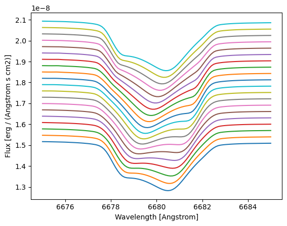
This plot illustrates the profile variations in the HeI \(\lambda6678\) line [2], arising from the surface velocity, temperature and geometry perturbations caused by the \(\ell=2\) pulsation mode. As is typical of prograde modes, bumps move from blue to red in the profile.

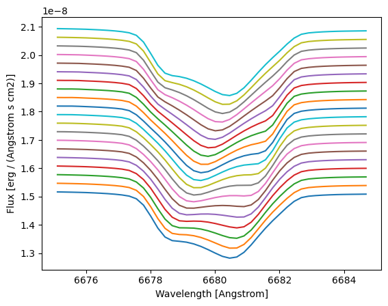
Advanced Usage

In addition to running PyKYLIE from the command line, there’s the option of interfacing with it from inside a Python script. This can allow more flexibility in configuring things. The following code reprises the calculation above, but now adopting a wavelength abcissa with constant resolving power \(\mathcal{R} \equiv \lambda/\Delta \lambda = 30,000\).

[3]:

import pymsg as pm
import pykylie as pk
import numpy as np

# Load the specgrid

specgrid = pm.SpecGrid('sg-BSTAR2006-high.h5')

specgrid.cache_limit = 2048 # To improve performance

# Set up bin wavelengths -- uniformly spaced in Delta log(lambda) to yield
# a constant resolving power

lam_min = 6675
lam_max = 6685
R = 30000

lam = np.exp(np.arange(start=np.log(lam_min), stop=np.log(lam_max), step=1/R))

# Set up mid-point wavelengths

lam_mid = 0.5*(lam[1:] + lam[:-1])

# Calculate and plot the spectra

plt.figure()

offset = 0

for i in range(20):

    # Read the BRUCE model

    model = pk.read_bruce_model(f'model-{i+1:03d}')

    # Evaluate the flux

    flux = pk.integrate_flux(model, specgrid, lam, x_add={'Z/Zo': 1.0})

    # Plot the flux

    plt.plot(lam_mid, flux+offset)

    # Update the offset (for stacking the spectra vertically)

    offset += flux[0]*0.02

plt.xlabel('Wavelength [Angstrom]')
plt.ylabel('Flux [erg / (Angstrom s cm2)]')

[3]:

Text(0, 0.5, 'Flux [erg / (Angstrom s cm2)]')

footnote